12 Exploring Advanced Neural Networks: Instance Segmentation

Overview

In the previous chapters, we learned how neural networks can recognize patterns in data, classify images, and even make pixel-wise predictions. But so far, our models could only tell what is in an image, but not where it is or what exact shape it has.

This chapter takes the next step. We’ll explore how neural networks evolved from simple classifiers into advanced models that can detect and outline every object in a scene, a task known as instance segmentation.

Think of it as moving from naming objects to understanding them in context.
For example, if a photo shows three dogs playing in the park, a classification network can tell you “there are dogs”.
An object-detection model goes further: “there are three dogs, each at these locations”.
An instance-segmentation model goes even further: “here are the three dogs and here are the exact pixels that belong to each one”.

In this section, you will:

Understand the difference between classification, object detection, semantic segmentation, and instance segmentation.
Learn how all these tasks share the same building blocks, input, feature extractor, and output, but differ in how those blocks are connected.
Follow the historical path of neural networks from R-CNN¹ → Fast R-CNN² → Faster R-CNN³ → Mask R-CNN⁴, seeing how each new design solved a real problem from the previous one.

By the end, you’ll see that advanced models aren’t mysterious or built from scratch. They’re the result of asking new questions and tweaking familiar parts of the same network structure you already know.

Quick Thought

Every time researchers faced a limitation, for example, “it’s too slow,” “it misses small objects,” “it can’t tell shapes apart”, they modified one of the three core components: input, feature extractor, or output.

As you read, try guessing which component each innovation changes!

12.1 What is instance segmentation?

Source: https://manipulation.csail.mit.edu/segmentation.html

Before diving into architectures, let’s first understand the concepts.

Computer vision has several “levels of understanding”, and each answers a slightly different question about an image.

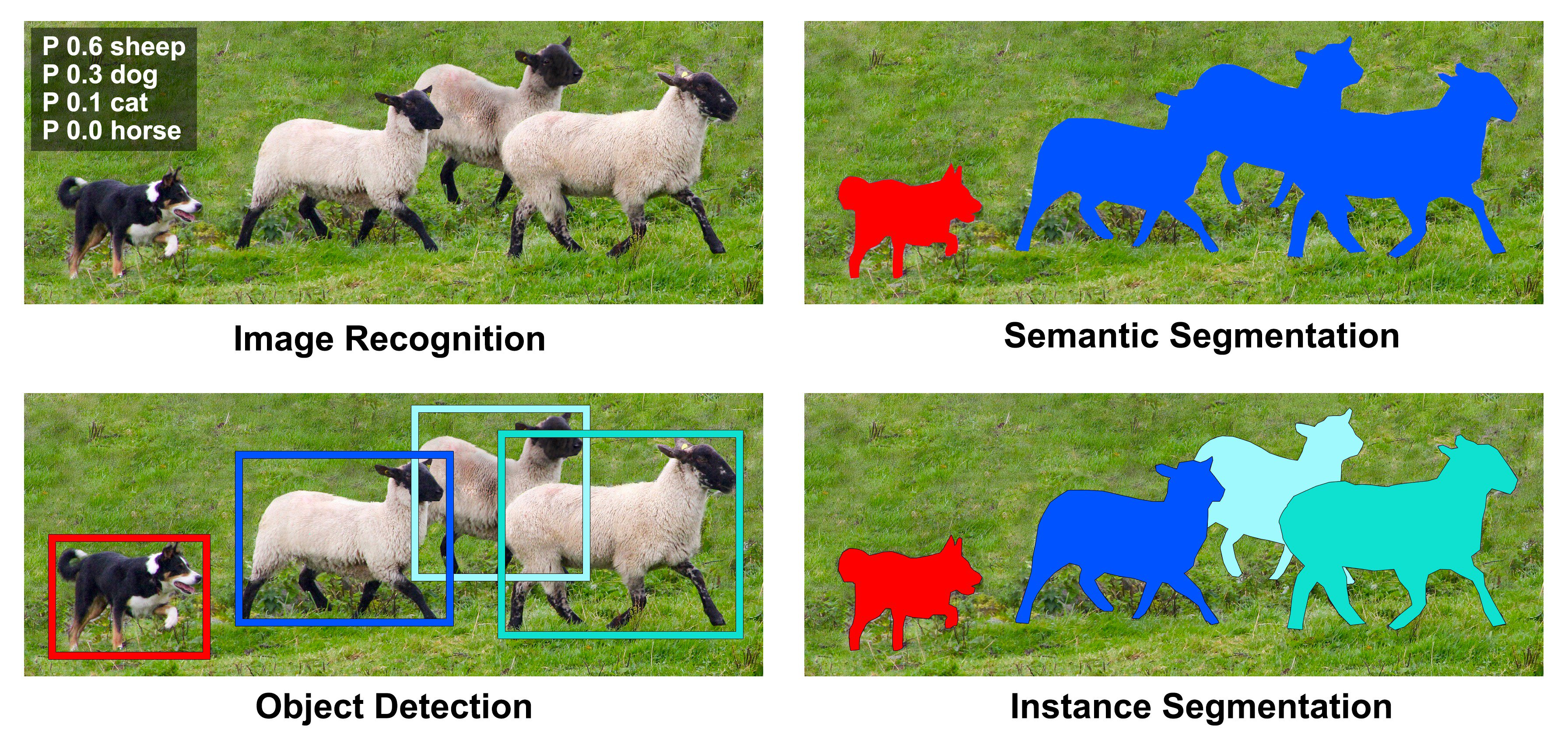
Task	What it asks	What the model outputs	Example thought
Image Classification	What kinds of objects are in this image?	One label per image	“This picture contains sheep.”
Object Detection	Where are those objects?	Bounding boxes + labels	“There are three sheep there and a dog here.”
Semantic Segmentation	Which class does each pixel belong to?	Pixel-wise class map	“Color every sheep pixel blue, every dog pixel red.”
Instance Segmentation	Which exact pixels belong to each individual object?	A mask + label for each instance	“Here are three separate sheep and a dog, each with its own outline.”

Instance segmentation therefore combines the strengths of object detection and semantic segmentation. It both detects objects (like detection) and delineates them (like segmentation). The result is a collection of colored masks, each describing one distinct instance of an object.

Key Idea

Instance segmentation tells the model: Don’t just find all the cats, tell me which pixels belong to Cat #1, Cat #2, and Cat #3.

Behind the scenes, this requires the model to learn fine-grained spatial details while still recognizing object categories. It’s a bit like tracing a outline after recognizing the object’s identity.

Quick Thought

Think of an example in your field:

Would you care the distinction between the different instances of the same object, or just the presence of the object? Would you rather have a box around a region, or the exact outline of that region’s shape?

That choice usually determines which task you need to solve.

12.2 Why Does It Matter?

Now that we know what instance segmentation is, let’s ask a simple question: why go through all that extra effort?

After all, drawing precise masks for every object sounds expensive and complex. But for many real-world problems, those extra pixels make a big difference.

1. Fine-grained precision

Bounding boxes only tell where an object roughly is. Instance segmentation tells exactly which pixels belong to it. That’s crucial whenever shape, size, or boundaries matter. For example, measuring a tumor, estimating crop coverage, or mapping glacial melt ponds.

2. Distinguishing look-alikes

Semantic segmentation colors all sheep the same color, as if they’re one big flock. Instance segmentation separates each sheep into its own mask. This distinction lets us count, track, and compare individuals, which is essential for crowd analysis, wildlife monitoring, or object-by-object statistics.

3. Enabling interaction

In robotics, augmented reality, or autonomous driving, systems must know where one object ends and another begins. With pixel-accurate masks, robots can grasp, avoid, or label objects more safely and reliably. Likewise, AR apps can anchor digital objects precisely on real-world surfaces.

Applications in the Wild

Field	How instance segmentation helps
🧬 Medical imaging	Identifies and measures individual organs, lesions, or cells with pixel-level accuracy ⁵.
🤖 Robotics & automation	Allows robots to perceive and interact with separate objects in cluttered scenes ⁶.
🌍 Environmental monitoring	Maps terrain features such as permafrost polygons or vegetation patches for change detection ⁷ ⁸.

Quick Thought

In your own research or projects, where would pixel-level detail unlock new insight?

Try to picture the same task using only bounding boxes. What information would you lose?

Next, we’ll peek under the hood: how do models actually achieve these capabilities?

To answer that, we’ll revisit our three familiar friends: input, feature extractor, and output, and see how every “advanced” network is just a creative remix of those parts.

12.3 From Building Blocks to Advanced Networks

So far, we’ve seen what instance segmentation is and why it matters. Now, let’s look at how we can make a neural network actually do it.

The good news?

Every deep learning model, no matter how complex its name sounds, is built from the same three ingredients you’ve already met:

Input adaptation: how data is prepared and passed into the network
Feature extractor: the main body of the model that learns patterns
Output adaptation: how the extracted information is translated into predictions

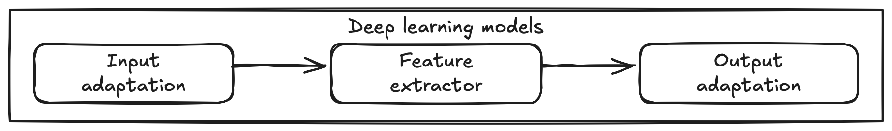
Think of it like a pipeline:

Input → Feature extractor → Output

Each part has its own job. When we move from classification to detection to segmentation, we don’t reinvent the pipeline; we just add new capabilities or modify one of the blocks to serve a different purpose.

Task	Input	Feature Extractor	Output
Classification	Image	CNN backbone (e.g., ResNet-50)	Class probabilities
Object Detection	Image	Same backbone	Bounding boxes + class labels
Instance Segmentation	Image	Same backbone	Masks + class labels

Notice how the feature extractor often stays the same, for example, ResNet-50, which you’ve already seen. What changes is mainly how we interpret those extracted features at the output.

This insight is powerful:

when researchers realized classification networks could already “see” complex features, they began reusing them for localization tasks: first for boxes, then for masks.

Each breakthrough (R-CNN, Fast R-CNN, Faster R-CNN, Mask R-CNN) simply tweaked one or more of these three blocks.

Key Idea

Advanced networks aren’t mysterious new inventions; they’re incremental upgrades built on the same foundation: input, features, output.

Quick Thought

Imagine you want your network to predict depth maps or object edges. Which component, input, feature extractor, or output, would you modify first?

Next, we’ll start from the most familiar example: a classification network, and see how small architectural changes gradually lead us toward instance segmentation.

12.4 Starting Point: Classification Networks

Before we leap into detection and segmentation, let’s anchor ourselves in something familiar: image classification.

At its core, a classification network answers a simple question:

“What category does this image belong to?”

For example, given a picture of fruit, the network might output:

apple: 0.85, banana: 0.10, orange: 0.05

Revisiting our three building blocks

Component	Role in classification	Example (ResNet-50)
Input	Accept an image (e.g., 3 RGB channels) and resize/normalize it for the model.	224 × 224 × 3 tensor
Feature Extractor	Learn rich visual patterns: edges → textures → shapes that describe the content.	Convolutional backbone of ResNet-50
Output Adaptation	Convert those features into class probabilities.	Final fully-connected layer + softmax

So, when we say “ResNet-50 backbone”, we’re really talking about the feature extractor block.

A quick look under the hood

Let’s load a pre-trained ResNet-50 from PyTorch and peek at its structure:

import torch
import torchvision.models as models

# Load the pre-trained ResNet-50 model
model = models.resnet50(pretrained=True)
print(model)

Click to view the whole architecture of ResNet-50

ResNet(
(conv1): Conv2d(3, 64, kernel_size=(7, 7), stride=(2, 2), padding=(3, 3), bias=False)
(bn1): BatchNorm2d(64, eps=1e-05, momentum=0.1, affine=True, track_running_stats=True)
(relu): ReLU(inplace=True)
(maxpool): MaxPool2d(kernel_size=3, stride=2, padding=1, dilation=1, ceil_mode=False)
(layer1): Sequential(
(0): BasicBlock(
(conv1): Conv2d(64, 64, kernel_size=(3, 3), stride=(1, 1), padding=(1, 1), bias=False)
(bn1): BatchNorm2d(64, eps=1e-05, momentum=0.1, affine=True, track_running_stats=True)
(relu): ReLU(inplace=True)
(conv2): Conv2d(64, 64, kernel_size=(3, 3), stride=(1, 1), padding=(1, 1), bias=False)
(bn2): BatchNorm2d(64, eps=1e-05, momentum=0.1, affine=True, track_running_stats=True)
)
(1): BasicBlock(
(conv1): Conv2d(64, 64, kernel_size=(3, 3), stride=(1, 1), padding=(1, 1), bias=False)
(bn1): BatchNorm2d(64, eps=1e-05, momentum=0.1, affine=True, track_running_stats=True)
(relu): ReLU(inplace=True)
(conv2): Conv2d(64, 64, kernel_size=(3, 3), stride=(1, 1), padding=(1, 1), bias=False)
(bn2): BatchNorm2d(64, eps=1e-05, momentum=0.1, affine=True, track_running_stats=True)
)
)
(layer2): Sequential(
(0): BasicBlock(
(conv1): Conv2d(64, 128, kernel_size=(3, 3), stride=(2, 2), padding=(1, 1), bias=False)
(bn1): BatchNorm2d(128, eps=1e-05, momentum=0.1, affine=True, track_running_stats=True)
(relu): ReLU(inplace=True)
(conv2): Conv2d(128, 128, kernel_size=(3, 3), stride=(1, 1), padding=(1, 1), bias=False)
(bn2): BatchNorm2d(128, eps=1e-05, momentum=0.1, affine=True, track_running_stats=True)
(downsample): Sequential(
(0): Conv2d(64, 128, kernel_size=(1, 1), stride=(2, 2), bias=False)
(1): BatchNorm2d(128, eps=1e-05, momentum=0.1, affine=True, track_running_stats=True)
)
)
(1): BasicBlock(
(conv1): Conv2d(128, 128, kernel_size=(3, 3), stride=(1, 1), padding=(1, 1), bias=False)
(bn1): BatchNorm2d(128, eps=1e-05, momentum=0.1, affine=True, track_running_stats=True)
(relu): ReLU(inplace=True)
(conv2): Conv2d(128, 128, kernel_size=(3, 3), stride=(1, 1), padding=(1, 1), bias=False)
(bn2): BatchNorm2d(128, eps=1e-05, momentum=0.1, affine=True, track_running_stats=True)
)
(layer3): Sequential(
(0): BasicBlock(
(conv1): Conv2d(128, 256, kernel_size=(3, 3), stride=(2, 2), padding=(1, 1), bias=False)
(bn1): BatchNorm2d(256, eps=1e-05, momentum=0.1, affine=True, track_running_stats=True)
(relu): ReLU(inplace=True)
(conv2): Conv2d(256, 256, kernel_size=(3, 3), stride=(1, 1), padding=(1, 1), bias=False)
(bn2): BatchNorm2d(256, eps=1e-05, momentum=0.1, affine=True, track_running_stats=True)
(downsample): Sequential(
(0): Conv2d(128, 256, kernel_size=(1, 1), stride=(2, 2), bias=False)
(1): BatchNorm2d(256, eps=1e-05, momentum=0.1, affine=True, track_running_stats=True)
)
)
(1): BasicBlock(
(conv1): Conv2d(256, 256, kernel_size=(3, 3), stride=(1, 1), padding=(1, 1), bias=False)
(bn1): BatchNorm2d(256, eps=1e-05, momentum=0.1, affine=True, track_running_stats=True)
(relu): ReLU(inplace=True)
(conv2): Conv2d(256, 256, kernel_size=(3, 3), stride=(1, 1), padding=(1, 1), bias=False)
(bn2): BatchNorm2d(256, eps=1e-05, momentum=0.1, affine=True, track_running_stats=True)
)
)
(layer4): Sequential(
(0): BasicBlock(
(conv1): Conv2d(256, 512, kernel_size=(3, 3), stride=(2, 2), padding=(1, 1), bias=False)
(bn1): BatchNorm2d(512, eps=1e-05, momentum=0.1, affine=True, track_running_stats=True)
(relu): ReLU(inplace=True)
(conv2): Conv2d(512, 512, kernel_size=(3, 3), stride=(1, 1), padding=(1, 1), bias=False)
(bn2): BatchNorm2d(512, eps=1e-05, momentum=0.1, affine=True, track_running_stats=True)
(downsample): Sequential(
(0): Conv2d(256, 512, kernel_size=(1, 1), stride=(2, 2), bias=False)
(1): BatchNorm2d(512, eps=1e-05, momentum=0.1, affine=True, track_running_stats=True)
)
)
(1): BasicBlock(
(conv1): Conv2d(512, 512, kernel_size=(3, 3), stride=(1, 1), padding=(1, 1), bias=False)
(bn1): BatchNorm2d(512, eps=1e-05, momentum=0.1, affine=True, track_running_stats=True)
(relu): ReLU(inplace=True)
(conv2): Conv2d(512, 512, kernel_size=(3, 3), stride=(1, 1), padding=(1, 1), bias=False)
(bn2): BatchNorm2d(512, eps=1e-05, momentum=0.1, affine=True, track_running_stats=True)
)
)
(avgpool): AdaptiveAvgPool2d(output_size=(1, 1))
(fc): Linear(in_features=512, out_features=1000, bias=True)
)
)

You’ll see a long list of convolutional layers grouped into four stages (layer1 to layer4), followed by:

(avgpool): AdaptiveAvgPool2d(output_size=(1, 1))
(fc): Linear(in_features=2048, out_features=1000, bias=True)

That last line, the fully connected (fc) layer, is the output adaptation. It converts the learned features into 1,000 ImageNet class scores.

Customizing for your own task

Suppose we want to classify images into 10 classes (say, 10 types of flowers). We keep the same input and feature extractor, but swap the output head:

import torch.nn as nn

# Replace the last layer with one suited for 10 classes
model.fc = nn.Linear(2048, 10)

That’s it! You’ve adapted a world-class backbone for your own dataset.

Key Idea

Classification models like ResNet-50 form the starting point for many advanced vision systems. Later, object-detection and segmentation models will reuse this exact feature extractor and simply modify what happens after it.

Quick Thought

If classification outputs a single label per image, what kind of modification might you need if you wanted to locate multiple objects instead?

Hint: the output block will need more than one prediction!

Next, we’ll follow that hint: evolving our classification network into models that can find and label multiple objects at once.

That journey begins with the first landmark in detection history: R-CNN.

12.5 The Evolution of Detection Models

Once we know how to classify an image, a natural next question appears:

“Can the model also tell me where each object is?”

This question led to one of the most important breakthroughs in computer vision: the evolution from simple classification to object detection, and eventually, instance segmentation.

Let’s trace this evolution through four key milestones:

R-CNN → Fast R-CNN → Faster R-CNN → Mask R-CNN.

Each model solves one major bottleneck of its predecessor.

12.5.1 R-CNN: The First Step

Imagine you’re a detective asked to locate every cat in a giant city photograph. You could inspect every pixel one by one, but that would take forever. Instead, you might first mark possible locations (windows, rooftops, gardens) and then zoom into each to decide whether a cat is really there.

That’s exactly the idea behind R-CNN (Region-based Convolutional Neural Network), proposed by Ross Girshick et al. in 2014 ⁹.

It was the first deep-learning model to detect and localize objects successfully.

Step 1: Propose candidate regions

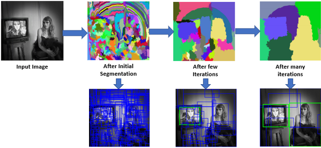
Illustration of Selective Search generating region proposals over an image. Source:geeksforgeeks

Before any neural network runs, R-CNN uses a separate algorithm called Selective Search¹⁰ to guess where objects might be. Think of it as a diligent assistant drawing ~2000 rectangles around promising areas of the image based on color, texture, and edges.

Each rectangle, called a region proposal, is a possible object.

Step 2: Extract features for each region

For every proposed region, we crop that portion of the image, resize it to a standard size, and feed it through a CNN (for example, AlexNet or ResNet).

The CNN acts as the feature extractor, producing a numerical fingerprint that describes the visual content.

# Pseudocode for R-CNN feature extraction
for region in selective_search(image):
    crop = resize(image[region], (224, 224))
    features = cnn(crop)

Because there are ~2000 regions, this step runs the CNN thousands of times per image. This is a key limitation we’ll revisit soon.

Step 3: Classify and refine boxes

Once we have the feature vector for each region:

A Support Vector Machine (SVM) predicts which class the region belongs to (cat, dog, car, …).
A linear regression model fine-tunes the coordinates of the bounding box to fit the object more tightly.

cls_score = svm(features)
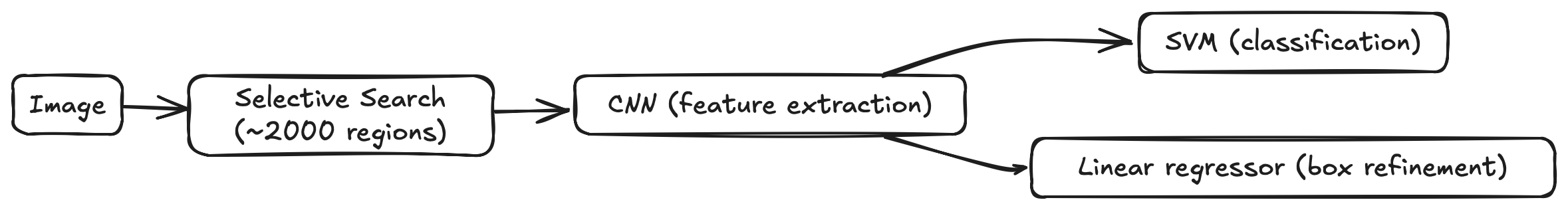
bbox = regressor(features)

So R-CNN’s output consists of bounding boxes and class labels.

Step 4: Combine the results

Finally, overlapping boxes are merged using Non-Maximum Suppression (NMS) ¹¹ so only the best one remains for each object.

The full pipeline looks like this:

How R-CNN fits into our three-block framework

Component	What R-CNN does
Input adaptation	Image + region proposals from Selective Search
Feature extractor	CNN applied separately to each region
Output adaptation	SVM + regressor for class + bounding box

What made R-CNN revolutionary

First to prove that deep CNN features outperform hand-crafted features (like HOG or SIFT) for object recognition.
Showed that localizing multiple objects could be framed as multiple independent classification problems.
Inspired the whole family of “Region-based CNNs” that followed.

But… it was painfully slow

~2000 regions × 1 CNN forward pass ≈ minutes per image.
Multi-stage training: CNN, then SVM, then regressor, then fine-tuning.
Heavy disk usage: each cropped region saved separately to disk before training.

The model worked, but not for real-time applications. Researchers loved its accuracy but craved speed.

Quick Thought

If every proposed region needs its own CNN pass, what could you change in the feature extractor to make this process faster?

Up next, we’ll see how Fast R-CNN answered exactly that question: by realizing we can share computation across all regions instead of repeating it thousands of times.

12.5.2 Fast R-CNN: Sharing Features

R-CNN worked, but it was painfully slow. Imagine our detective from earlier: instead of scanning one high-resolution map, they visit every single building in the city one by one. It works, but it’s exhausting.

Ross Girshick, the same researcher who created R-CNN, asked a simple but brilliant question in 2015:

“What if we extract features just once for the whole image, and reuse them for all regions?”

That idea became Fast R-CNN – a version that was not only faster but also simpler and more elegant.

Step-by-step walkthrough

Input: Feed the entire image into the CNN backbone (e.g., VGG16 or ResNet).
```
feature_map = cnn(image)
```
Region proposals: Use Selective Search to get ~2000 candidate regions (same as R-CNN). These are now rectangles in image coordinates.
Map regions onto the feature map: Each region is projected from image coordinates to the corresponding area on the feature map.
RoI Pooling: This is Fast R-CNN’s most clever trick. Because proposed regions vary in size, we can’t feed them directly into a fully connected layer. RoI Pooling crops the portion of the feature map corresponding to each region and pools it into a fixed spatial size (for example, 7×7).
```
for roi in proposals:
    roi_feat = roi_pool(feature_map, roi, output_size=(7, 7))
```
Classification and bounding box regression: Each RoI feature (7×7×C) is flattened and sent through two fully connected layers, producing:
- Class scores
- Bounding box refinements
```
cls_score, bbox = head(roi_feat)
```

Unified training and loss

Unlike R-CNN, which trained separate models (CNN → SVM → regressor), Fast R-CNN trains everything together using a multi-task loss:

\[ L = L_\text{cls} + \lambda L_\text{bbox} \]

\(L_\text{cls}\): classification loss (softmax cross-entropy)
\(L_\text{bbox}\): bounding box regression loss (smooth L1)

This end-to-end training makes the model both faster to train and more accurate.

What improved from R-CNN

Aspect	R-CNN	Fast R-CNN	Improvement
Feature extraction	Separate CNN per region	One CNN per image (shared)	🚀 10–20× faster
Training	Multi-stage (CNN, SVM, regressor)	Unified, single-stage	Simpler
Storage	Pre-compute region features	On-the-fly computation	No extra disk space
Accuracy	High	Higher (better end-to-end learning)	✔️

But one bottleneck remains…

Even though feature extraction became efficient, region proposals were still generated by the external Selective Search algorithm. Selective Search was CPU-based and slow. It took nearly two seconds per image.

So, while inference was much faster, it wasn’t yet real-time.

How Fast R-CNN fits into our three-block framework

Component	What changed from R-CNN
Input adaptation	Still uses region proposals (Selective Search), but processes one shared image feature map.
Feature extractor	Shared CNN backbone computes features once.
Output adaptation	Unified head with RoI Pooling + fully connected layers for classification and box regression.

Key Idea

Fast R-CNN taught us that most of the heavy computation in object detection could be shared.

It’s like realizing you don’t need to bake a separate cake for each guest. You just slice one big cake into pieces.

Quick Thought

If Selective Search is now the slowest part, what if we teach the network itself to generate region proposals automatically?

That question led directly to the next major leap: Faster R-CNN: a model that learns to propose its own regions, eliminating Selective Search altogether.

12.5.3 Faster R-CNN: End-to-End Detection

Our detective has gotten smarter.

In R-CNN, they searched every building; in Fast R-CNN, they looked at one satellite map and zoomed in on areas of interest.

But they’re still relying on a human assistant (Selective Search) to tell them where to look next and that assistant is slow.

So, in 2015, a new idea arrived:

“What if the network itself could learn where objects are likely to appear?”

This question gave birth to Faster R-CNN by Shaoqing Ren et al. (2015) ¹², the first truly end-to-end object-detection framework. Its secret weapon: the Region Proposal Network (RPN).

The key innovation: Region Proposal Network (RPN)

The RPN is a tiny neural network that slides over the shared feature map (produced by the CNN backbone) and proposes potential object regions automatically. In other words, the network learns to generate its own “Select me!” boxes.

Faster R-CNN pipeline: shared feature map feeding both the RPN and the detection head.

Step-by-step walkthrough

Feature extraction: As before, we start with a CNN backbone (e.g., ResNet-50 or VGG-16) that processes the entire image once:
```
feature_map = cnn(image)      # shared backbone
```
This feature map is now shared by two heads: the RPN (proposal generator) and the detection head (classifier + box regressor).
Generate anchors: At each location on the feature map, the model places a small set of anchor boxes – templates of different sizes and aspect ratios. You can think of them as little “nets” cast over the image, waiting to be adjusted.
```
anchors = generate_anchors(feature_map, scales=[128,256,512], ratios=[0.5,1,2])
```
Each anchor will be tested: “Does this anchor contain an object?”
Predict objectness and box offsets: The RPN slides a 3×3 convolutional window over the feature map. For each anchor, it outputs:
- an objectness score (probability that an object exists here), and
- a bounding-box offset to refine the anchor’s shape and position.
```
for anchor in anchors:
    obj_score, bbox_offset = rpn_head(feature_map, anchor)
```
After this step, the RPN has thousands of proposals with confidence scores.
Select top proposals: A post-processing step called Non-Maximum Suppression (NMS) removes redundant boxes. Typically, the top ~2000 highest-scoring proposals (300 in practice) are kept.
```
proposals = nms(anchors, obj_score, top_k=300)
```
These proposals replace the old Selective Search regions.
RoI Pooling → Detection Head: Each proposed region is cropped (via RoI Pooling or RoI Align) from the shared feature map and fed into the detection head — the same classification + box regression module introduced in Fast R-CNN:
```
for roi in proposals:
    roi_feat = roi_pool(feature_map, roi)
    cls_score, bbox = head(roi_feat)
```

Training as one network

Both the RPN and the detection head share the same convolutional features and are trained jointly. The total loss combines RPN loss + detection loss:

\[ L = L_\text{RPN-cls} + L_\text{RPN-bbox} + L_\text{Det-cls} + L_\text{Det-bbox} \]

This means the entire system, from pixels to final boxes, learns together.

Why it matters

Aspect	Fast R-CNN	Faster R-CNN	Improvement
Region proposals	Hand-crafted Selective Search (CPU)	Learned Region Proposal Network (GPU)	🚀 100× faster
End-to-end training	Partial (Selective Search external)	Fully integrated	Unified
Speed	~2 FPS on GPU	~10 FPS on GPU	Real-time possibility
Accuracy	High	Higher (learned proposals fit better)	✔️

The RPN made object detection practical for real-world systems and set the foundation for everything that came after, including instance segmentation.

How Faster R-CNN fits into our three-block framework

Component	What changed from Fast R-CNN
Input adaptation	Added Region Proposal Network to generate anchors and proposals internally.
Feature extractor	Shared backbone features used by both RPN and detection head.
Output adaptation	Two branches (classification + regression) refine proposals end-to-end.

A mental picture

It’s as if our detective now works with a drone that automatically highlights potential objects from above. The detective still classifies them (cat, dog, car…), but no longer wastes time choosing where to look.

Key Idea

Faster R-CNN solved the last major bottleneck by teaching the network to propose its own regions. The result is a fully trainable system that detects objects with both speed and precision.

Quick Thought

If the model can now predict object locations and labels efficiently, what extra branch would you add to also predict each object’s exact shape?

Up next is exactly that extension: Mask R-CNN, which builds on Faster R-CNN to perform full instance segmentation, adding a mask prediction head for pixel-level detail.

12.6 Mask R-CNN: From Detection to Segmentation

At this point, our detective is lightning-fast. Thanks to Faster R-CNN, they can spot every object in a scene almost in real time. But there’s still one question left unanswered:

“Can you draw the precise outline of each object, not just a box around it?”

This challenge led to Mask R-CNN by Kaiming He et al. (2017) ¹³, a direct successor to Faster R-CNN that added the ability to perform instance segmentation, predicting a mask for every detected object.

Mask R-CNN didn’t reinvent the wheel; it simply bolted one more well-designed component onto the same framework.

The key idea: Add a mask branch

Faster R-CNN already produced bounding boxes and class labels. Mask R-CNN adds a third parallel branch that predicts a binary mask, a small image showing which pixels belong to the detected object.

Mask R-CNN: shared backbone → RPN → RoI Align → three heads (cls / bbox / mask).

So for each proposed region, the model now outputs:

Class label
Bounding box
Segmentation mask

All three are trained together in one network.

Step-by-step walkthrough

1. Shared feature extraction

As before, the entire image is passed through a backbone (ResNet-50, ResNet-101, etc.) to produce a feature map shared by all heads.

feature_map = backbone(image)

The RPN (Region Proposal Network) then proposes candidate boxes from this feature map — identical to Faster R-CNN.

2. RoI Align: precise region cropping

Fast / Faster R-CNN used RoI Pooling to crop regions of interest, but pooling involved rounding coordinates to integers, which introduced slight misalignments. Those pixel-level shifts are small for detection, but catastrophic for mask accuracy.

RoI Align fixes this by using bilinear interpolation instead of quantization, preserving exact spatial locations.

roi_feat = roi_align(feature_map, roi, output_size=(14,14))

Each RoI now corresponds perfectly to its true image region.

3. Three parallel heads

Once features are extracted, they’re sent into three separate branches:

Head	Output	Purpose
Classification head	Class scores	Identify what the object is
Bounding box head	Box offsets	Refine position + size
Mask head	Pixel mask (28×28)	Predict which pixels belong to the object

cls_score, bbox = det_head(roi_feat)
mask_logits = mask_head(roi_feat)        # small conv decoder
mask = sigmoid(mask_logits)

Each mask head is a lightweight CNN (often 4 conv layers) that outputs one binary mask per class.

4. Training the mask branch

Only the RoIs corresponding to foreground objects are used for mask training. The loss is a pixel-wise binary cross-entropy between predicted and true masks:

\[ L_\text{mask} = \frac{1}{N} \sum_{i} \text{BCE}(M_i^\text{pred}, M_i^\text{gt}) \]

The total loss combines all three branches:

\[ L = L_\text{cls} + L_\text{bbox} + L_\text{mask} \]

Everything is trained together, end-to-end.

How Mask R-CNN fits into our three-block framework

Component	What changed from Faster R-CNN
Input adaptation	Same as Faster R-CNN (image → feature map → RPN proposals)
Feature extractor	Shared backbone + RoI Align for precise spatial features
Output adaptation	Added a mask branch (28×28 pixel-wise prediction per instance)

Code peek: using Mask R-CNN in PyTorch

PyTorch makes this architecture accessible with just a few lines:

import torchvision.models.detection as detection

# Load a pretrained Mask R-CNN (ResNet-50 backbone)
model = detection.maskrcnn_resnet50_fpn(pretrained=True)
model.eval()

# Forward pass
predictions = model([image])     # image: Tensor [C,H,W]

Each prediction contains:

boxes – bounding boxes
labels – class IDs
scores – confidence values
masks – [ N × 1 × H × W ] tensor of pixel-level masks

You can threshold and overlay these masks to visualize segmentation results.

Why it matters

Aspect	Faster R-CNN	Mask R-CNN	Improvement
Output	Boxes + labels	Boxes + labels + masks	🟢 Pixel-level precision
Alignment	RoI Pooling (rounding)	RoI Align (interpolation)	🟢 No quantization error
Capability	Object detection	Instance segmentation	🟢 New dimension of understanding

A mental picture

Our detective can now not only say

“There’s a cat at these coordinates,” but also trace its exact fur outline, whiskers and all. No more rough boxes — just precise boundaries.

Key Idea

Mask R-CNN is Faster R-CNN with one extra branch and a more careful alignment step.

A tiny change in architecture enabled a huge leap in capability, from detecting objects to understanding their shapes.

Quick Thought

Which of the three components, input, feature extractor, or output, did Mask R-CNN change most significantly?

How might you extend the same idea to tasks like keypoint detection or depth estimation?

Mask R-CNN set a template for modern segmentation and instance-aware vision models.

Next, we’ll step back and see how all these models, from R-CNN to Mask R-CNN, fit together in one unified story.

12.7 Putting It All Together

We’ve traveled quite a distance from recognizing what is in an image to outlining where and what shape each object takes. Let’s step back and see how every step in this journey fits together.

From classification to instance segmentation

Generation	Year	Key Idea	Input Adaptation	Feature Extractor	Output Adaptation
Classification Network	2012 (AlexNet)	Recognize categories in whole images.	Full image	CNN backbone (e.g., ResNet)	Class probabilities
R-CNN	2014	Detect objects using region proposals + independent CNNs.	Selective Search regions	Separate CNN per region	SVM + regressor
Fast R-CNN	2015	Share convolutional features + RoI Pooling.	Selective Search	One shared CNN per image	Unified head for classification + bbox
Faster R-CNN	2015	Learn region proposals via Region Proposal Network (RPN).	RPN (anchors + proposals)	Shared backbone (CNN + FPN)	End-to-end classification + bbox
Mask R-CNN	2017	Add mask prediction head for pixel-level segmentation.	Same as Faster R-CNN	Shared backbone + RoI Align	Three parallel heads (cls, bbox, mask)

Visual timeline

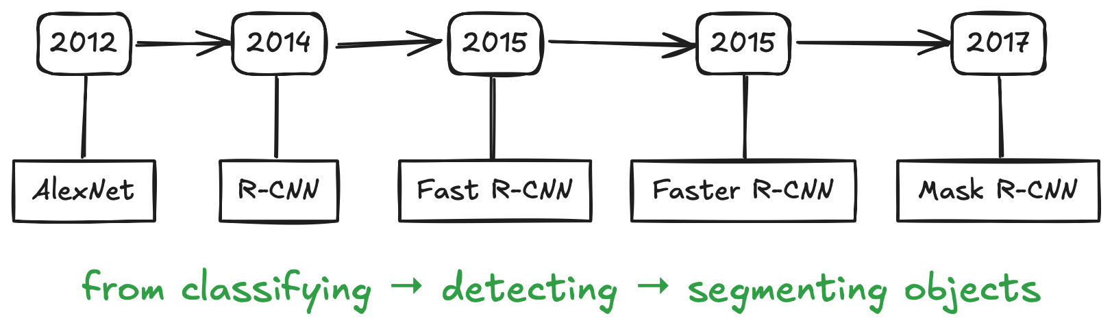
Each new architecture didn’t replace the old; it refined one of the three building blocks to solve a real bottleneck:

Component Modified	Examples	Goal
Input adaptation	R-CNN (Selective Search), Faster R-CNN (RPN)	Generate or refine region proposals
Feature extractor	Fast R-CNN (shared CNN)	Reuse computation efficiently
Output adaptation	Mask R-CNN (mask head)	Predict more detailed outputs

A recurring pattern

Every innovation begins by asking: “What can’t the current model do well?” and then tweaking one of the three parts to fix it.

This pattern defines much of deep learning progress:

Better inputs → more context (multi-scale images, temporal frames, extra bands).
Stronger feature extractors → deeper, more efficient backbones (ResNet, Swin, ViT).
Richer outputs → new tasks (masks, depth, keypoints, motion).

Once you start thinking in this modular way, “advanced models” stop feeling like magic, they become creative recombinations of familiar ideas.

A unifying view

Unified view of R-CNN family — single backbone feeding multiple heads.

All four models share the same skeleton:

A backbone that learns features.
A proposal mechanism (external or learned).
One or more heads that interpret those features for different tasks.

The Mask R-CNN simply made that skeleton multi-talented — detecting, classifying, and segmenting all at once.

Key Idea

From R-CNN to Mask R-CNN, progress wasn’t about adding complexity for its own sake. It was about removing redundancy, integrating stages, and expanding output richness all while keeping the same underlying logic.

Quick Thought

If you were to design “the next R-CNN,” what might you change? Would you feed richer inputs (e.g., multispectral data)? Use a new feature extractor (e.g., transformer backbone)? Or predict new outputs (e.g., elevation maps, uncertainty masks)?

12.8 Reflection and Discussion

Let’s pause and reflect on what we’ve learned.

From R-CNN to Mask R-CNN, each step wasn’t random, it was a logical response to a real problem. This mindset is what separates using deep learning from understanding it.

Looking back

Model	Challenge it solved	Core idea introduced
R-CNN	How can a CNN detect multiple objects?	Apply CNN to region proposals (Selective Search)
Fast R-CNN	Why is R-CNN so slow?	Share one feature map for all regions
Faster R-CNN	Can we remove the slow proposal step?	Learn proposals via Region Proposal Network (RPN)
Mask R-CNN	Can we see object shapes, not just boxes?	Add a mask head + precise RoI Align

Notice how each question leads to an architectural insight and how every model keeps the same foundation:

input adaptation → feature extractor → output adaptation.

Reflection Prompts

Quick Thought

Imagine you are designing your own vision model.

Which component (input, feature, output) would you modify first?
What kind of task would that change enable (for example, predicting object depth or motion)?

Challenge

Sketch your own “R-CNN++”:

Keep the same three blocks.
Add one new branch or data source.
Write a one-sentence explanation of why it improves the model. You don’t need code, just reasoning.

Discussion

Why do you think so many breakthroughs (R-CNN → Mask R-CNN → modern detectors) reused the same ideas instead of starting from scratch?

What does this tell us about how innovation happens in deep learning?

Key takeaway

Deep learning progress often follows a simple pattern:

Question → Limitation → Innovation

Each new model asks:

“What can’t the current system do well?” and then modifies one of the core building blocks to fix it.

When you look at architectures through this lens, they stop feeling like black boxes, and start looking like creative engineering solutions to everyday problems.

Overview

12.1 What is instance segmentation?

12.2 Why Does It Matter?

1. Fine-grained precision

2. Distinguishing look-alikes

3. Enabling interaction

Applications in the Wild

12.3 From Building Blocks to Advanced Networks

12.4 Starting Point: Classification Networks

Revisiting our three building blocks

A quick look under the hood

Customizing for your own task

12.5 The Evolution of Detection Models

12.5.1 R-CNN: The First Step

Step 1: Propose candidate regions

Step 2: Extract features for each region

Step 3: Classify and refine boxes

Step 4: Combine the results

How R-CNN fits into our three-block framework

What made R-CNN revolutionary

But… it was painfully slow

12.5.2 Fast R-CNN: Sharing Features

The key idea: share the feature map

Step-by-step walkthrough

Unified training and loss

What improved from R-CNN

But one bottleneck remains…

How Fast R-CNN fits into our three-block framework

12.5.3 Faster R-CNN: End-to-End Detection

The key innovation: Region Proposal Network (RPN)

Step-by-step walkthrough

Training as one network

Why it matters

How Faster R-CNN fits into our three-block framework

A mental picture

12.6 Mask R-CNN: From Detection to Segmentation

The key idea: Add a mask branch

Step-by-step walkthrough

1. Shared feature extraction

2. RoI Align: precise region cropping

3. Three parallel heads

4. Training the mask branch

How Mask R-CNN fits into our three-block framework

Code peek: using Mask R-CNN in PyTorch

Why it matters

A mental picture

12.7 Putting It All Together

From classification to instance segmentation

Visual timeline

A recurring pattern

A unifying view

12.8 Reflection and Discussion

Looking back

Reflection Prompts

Key takeaway